R Programming Language - Overview

The R programming language is an important tool for development in the numeric analysis and machine learning spaces. With machines becoming more important as data generators, the popularity of the language can only be expected to grow. R first appeared in the 1990s and has served as an implementation of the S statistical programming language.

Why use R?

R is a programming language and software environment for statistical analysis, graphics representation, and reporting. Below are the reasons, why you should use R:

• R is an object-oriented programming environment, much more than most other statistical software packages
• R is a comprehensive statistical platform, offering all manner of data-analytic techniques – any type of data analysis can done in R
• R has state-of-the-art graphics capabilities- visualize complex data
• R is a powerful platform for interactive data analysis and exploration
• R functionality can be integrated into applications written in other languages, including C++, Java, Python, PHP, SAS, and SPSS
• R runs on a wide array of platforms, including Windows, Unix and Mac OS X.
• R is extensible; can be expanded by installing “packages”

Is R programming an easy language to learn?

All you need is data and a clear intent to draw a conclusion based on analysis of that data. In fact, R is built on top of the language that was originally intended as a programming language that would help the student learn to program while playing around with data. However, programmers that come from a Python, PHP, or Java background might find R quirky and confusing at first. The syntax that R uses is a bit different from other common programming languages.

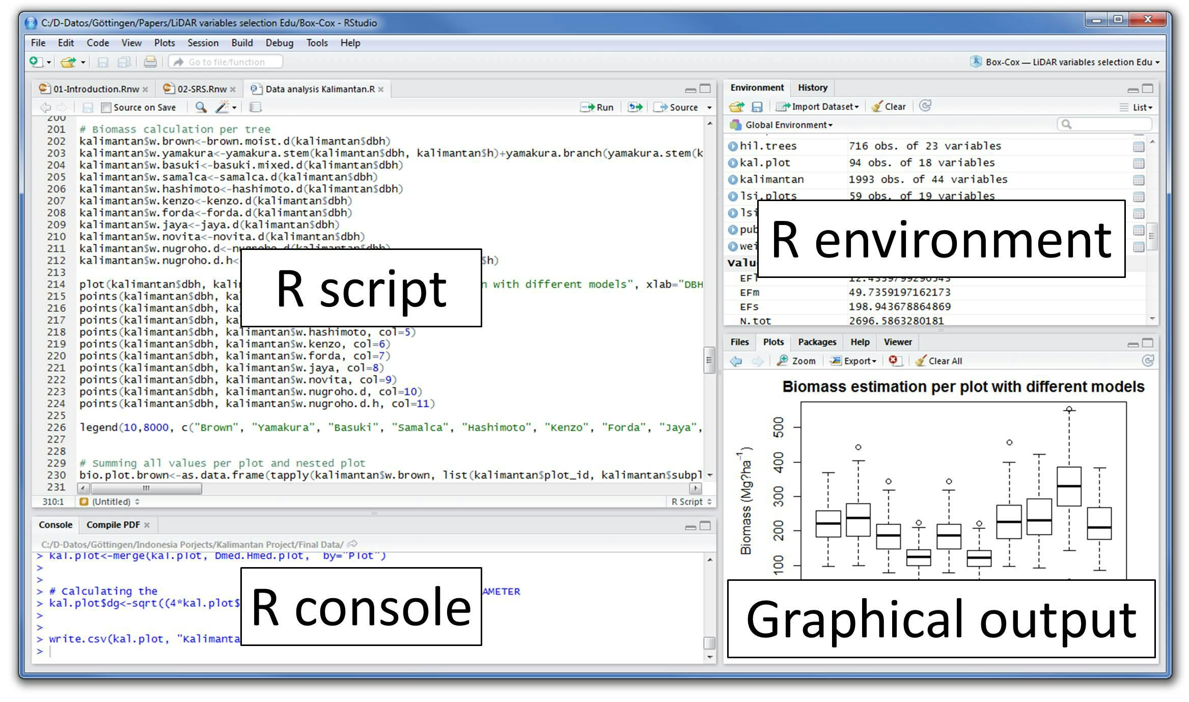
Head over to R Studio and download the setup for your OS(Linux, Mac, Windows) and you are ready to work with R language...

Getting started with R language

R is a dynamically typed language, meaning that variables need not be pre-declared with a specific data type. Rather, variables take on whatever type is necessary, based on the value assigned to them. The following statements show some examples:

num1 <- 5.5
6 -> num2
print(num1)  # 5.5
print(num2)  # 6

num2 = "Two"
print(num2)  # "Two"

In R, the assignment operator is <- or -> (although the usual = operator is also supported). To check the data type of variables, use the typeof() function:

print(typeof(num1))  # "double"
print(typeof(num2))  # "character"

You can also perform multiple assignments in a single statement, like this:

num2 = 6
num4 <- num3 <- num2
print(num3)                  # 6
print(num4)                  # 6

One common misconception when dealing with string variables is to assume that the length() function returns the length of the string, as the following example illustrates:

str = "This is a string"
print(str)           # "This is a string"
print(length(str))   # 1

Interestingly, the length() function returns a 1 for the above example. This is because the length() function returns the length of vectors

In R, you can get more information about a specific function by using the print() function. For example:

print(exp)
# function (x)  .Primitive("exp")

The above code statement shows the exp() function, which takes in a single argument and returns a primitive result. Here's another example:

print(log)
# function (x, base = exp(1))  .Primitive("log")

The log() function takes in two arguments. The second argument has a default value of exp(1) and the function returns a primitive result. You can now see how to call the log() function using the various combinations of arguments:

print(log(10))                # 2.302585
print(log(10, base=exp(1)))   # 2.302585
print(log(10, base=10))       # 1
print(log(10, 10))            # 1
print(log(base=exp(1), x=10)) # 2.302585
print(log(base=exp(1), 10))   # 2.302585

Note that you can swap the order of the arguments if you specify the argument names. This is very useful as it makes the function calls much more self-explanatory. They are also some scientific and mathematical functions in R:

print(sin(90))                # 0.8939967
print(cos(180))               # -0.5984601
print(tan(270))               # -0.1788391

print(factorial(6))           # 720

print(round(3.14))            # 3
print(round(3.145, 2))        # 3.15

There is a lot more than these basic commands such as dealing with vectors, making decisions, creating your own functions, and many more.

In the upcoming blogs, will have these topics introduced in depth. I hope I did give enough reasons to make your own decision to choose between programming language ❤️. All the best :)